pal <- RColorBrewer::brewer.pal(4, "PuBuGn")
color_ramp <- colorRampPalette(pal, space = "Lab") Introducing qualpalr
r
data visualization
qualpalr
Let me introduce qualpalr: an R package that generates qualitative color palettes with distinct colors using color difference algorithms.
Introduction
With the advent of colorbrewer there now exists good options to generate color palettes for sequential, diverging, and qualitative data. In R, these palettes can be accessed via the popular RColorBrewer package. Those palettes, however, are limited to a fixed number of colors. This isn’t much of a problem for sequential of diverging data since we can interpolate colors to any range we desire:
There is not, however, an analogue for qualitative color palettes that will get you beyond the limits of 8–12 colors of colorbrewer’s qualitative color palettes. There is also no customization in colorbrewer. Other R packages, such as colorspace offer this, but they are primarily adapted to sequential and diverging data – not qualitative data.
This is where qualpalr comes in. qualpalr provides the user with a convenient way of generating distinct qualitative color palettes, primarily for use in R graphics. Given n (the number of colors to generate), along with a subset in the hsl color space (a cylindrical representation of the RGB color space) qualpalr attempts to find the n colors in the provided color subspace that maximize the smallest pairwise color difference. This is done by projecting the color subset from the HSL color space to the DIN99d space. DIN99d is (approximately) perceptually uniform, that is, the euclidean distance between two colors in the space is proportional to their perceived difference.
Examples
qualpalr relies on one basic function, qualpal(), which takes as its input n (the number of colors to generate) and colorspace, which can be either
- a list of numeric vectors
h(hue from -360 to 360),s(saturation from 0 to 1), andl(lightness from 0 to 1), all of length 2, specifying a min and max, or - a character vector specifying one of the predefined color subspaces, which at the time of writing are pretty, pretty_dark, rainbow, and pastels.
library(qualpalr)
pal <- qualpal(
  n = 5,
  list(
    h = c(0, 360),
    s = c(0.4, 0.6),
    l = c(0.5, 0.85)
  )
)

# Adapt the color space to deuteranopia
pal <- qualpal(n = 5, colorspace = "pretty", cvd = "deutan")
The resulting object, pal, is a list with several color tables and a distance matrix based on the din99d color difference formula.
pal----------------------------------------
Colors in the HSL color space
Hue Saturation Lightness
#73CA6F 117 0.46 0.61
#D37DAD 327 0.50 0.66
#C6DBE8 203 0.42 0.84
#6C7DCC 229 0.48 0.61
#D0A373 31 0.50 0.63
----------------------------------------
DIN99d color difference distance matrix
#73CA6F #D37DAD #C6DBE8 #6C7DCC
#D37DAD 28
#C6DBE8 19 21
#6C7DCC 27 19 19
#D0A373 19 18 20 25Methods for pairs and plot have been written for qualpal objects to help visualize the results.
plot(pal)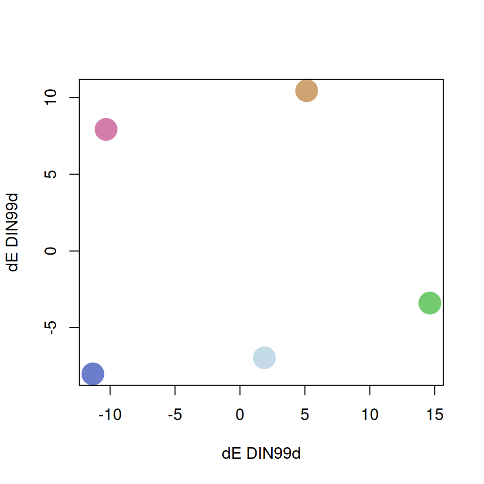
pairs(pal, colorspace = "DIN99d", asp = 1)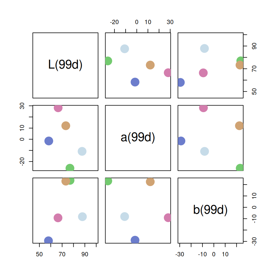
The colors are normally used in R by fetching the hex attribute of the palette. And so it is straightforward to use the output to, say, color the provinces of France (Figure 3).
library(maps)
map("france", fill = TRUE, col = pal$hex, mar = c(0, 0, 0, 0))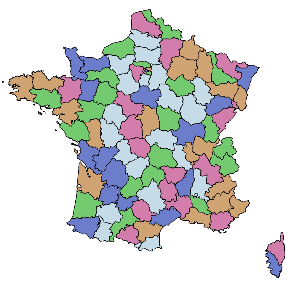
Details
qualpal begins by generating a point cloud out of the HSL color subspace provided by the user, using a quasi-random torus sequence from randtoolbox. Here is the color subset in HSL with settings h = c(-200, 120), s = c(0.3, 0.8), l = c(0.4, 0.9).
The function then proceeds by projecting these colors into the sRGB space (Figure 5).
It then continues by projecting the colors, first into the XYZ space, then CIELab (not shown here), and then finally the DIN99d space (Figure 6).
The DIN99d color space (Cui et al. 2002) is a euclidean, perceptually uniform color space. This means that the difference between two colors is equal to the euclidean distance between them. We take advantage of this by computing a distance matrix on all the colors in the subset, finding their pairwise color differences. We then apply a power transformation (Huang et al. 2015) to fine tune these differences.
To select the n colors that the user wanted, we proceed greedily: first, we find the two most distant points, then we find the third point that maximizes the minimum distance to the previously selected points. This is repeated until n points are selected. These points are then returned to the user; below is an example using n = 5.
Color specifications
At the time of writing, qualpalr only works in the sRGB color space with the CIE Standard Illuminant D65 reference white.
Future directions
The greedy search to find distinct colors is crude. Particularly when searching for few colors, the greedy algorithm will lead to sub-optimal results. Other solutions to finding points that maximize the smallest pairwise distance among them are welcome.
Thanks
Bruce Lindbloom’s webpage has been instrumental in making qualpalr. Also thanks to i want hue, which inspired me to make qualpalr.
References
Cui, G., M. R. Luo, B. Rigg, G. Roesler, and K. Witt. 2002. “Uniform Colour Spaces Based on the DIN99 Colour-Difference Formula.” Color Research & Application 27 (4): 282–90. https://doi.org/cz7764.
Huang, Min, Guihua Cui, Manuel Melgosa, Manuel Sánchez-Marañón, Changjun Li, M. Ronnier Luo, and Haoxue Liu. 2015. “Power Functions Improving the Performance of Color-Difference Formulas.” Optics Express 23 (1): 597. https://doi.org/gcsk6f.